Adapting UAV Control for Latency

This article discusses my undergraduate thesis project, working on flying drones with latency and the development of a latency compensation system to allow flight when a latency is present. I’d like to start off this article with a bit of a teaser; the following video shows operation of a micro quadrotor UAV in rate mode with a control latency of 500ms using the latency compensation system I have created. Without the latency compensation system, the UAV is barely controllable/uncontrollable with a 500ms latency. Keep reading to find out exactly what’s going on and why it works!

Background

Latency refers to a time delay. The most obvious source of latency when operating a UAV is transmission delay (packet routing within a network and signals travelling distance at finite speed), though processing delay (such as when de/en-coding a HD video stream for transmission) can also produce latency. Manufacturers of video link systems have for some time been working to reduce the latency of their video transmission systems. Operators of UAVs via satellite connection use control abstraction, which changes an operator’s instructions to be higher level (e.g. increasing levels of control abstraction: “Deflect Ailerons”, “Roll to the Left”, “Turn Left”, “Move to Waypoint”, “Survey Region”).

My work has been inspired by the Aerial International Racing of Unmanned Systems (AIRUS) student project here at The University of Sydney (collaborating with a student team at Texas A&M University). For the AIRUS project, the objective was to fly a UAV in Texas while the operator sits in Sydney, and vice versa. Because the intention was to permit a race between pilots, manual control was a requirement. Commands from the operator and feedback from the UAV (a video stream) was sent using the internet. Under this arrangement, the majority of the control latency is produced by the internet ping time between the two locations. The ping time is the time taken for a packet (a packet is to the internet as a stamped envelope is to the postal system) to be sent from Sydney to Texas and then from Texas back to Sydney, so it is a round trip time.

The AIRUS project saw success in achieving control over the distance, however the latency meant that control of the UAV was extremely difficult. The focus of my thesis project was not to reduce this latency (ping times place a lower limit on the latency) but given that it exists find some way to deal with it that puts the operator on the stick rather than typing waypoints in.

Concept

There is a strong analogy to be drawn between “lag” compensation in multiplayer videogames and latency compensation when operating UAVs. With a UAV, an operator sends commands to effect desired changes in the vehicle state, which alters the feedback that the vehicle then sends to the operator. With a multiplayer videogame, a player sends commands to effect desired changes in the game state, which alters the feedback that the game then sends to the player. Multiplayer videogames must handle a wide range of latencies and circumstances as well as a large number of players. The topic is fascinating and well developed. Use of compensatory systems has been so widespread for so long that players have created comedic renditions of some of the weirdness it can produce:

The UAVs case I am interested in has a single pilot operating a single UAV, which is substantially simpler than the video game case. The paper that everyone cites on videogame lag compensation is Yahn Bernier’s 2001 paper on the topic. The paper discusses a number of techniques and how they apply to various videogame formats, most relevant of which is client side prediction. Bernier writes

A fantastic online demonstration (as well as detailed description of the client-server architecture used in videogames to effect client side prediction) can be found on Gabriel Gambetta’s website.

If we apply the client side prediction concept to a UAV, then the goal of a latency compensator would be to assume the commands being given will reach the vehicle and alter the vehicle state and then augment the feedback that is displayed to the operator (“prediction” on Gambetta’s site). The augmentation must be temporary, as the feedback will reflect the inputs received prior to the time that it is generated (handled by “reconciliation” on Gambetta’s site).

Mathematical Specifics

Now that we’ve a concept to try applying we can start working out the specifics for the UAV case. Diagrammatically, the problem we are dealing with looks something like the following.

If we are the operator at the current time t_n then we are viewing the feedback that was generated when the command from t_n – 2τ arrived at the vehicle. Here the round trip delay time is 2τ, and you could assume that the latency each way is τ if you like (though only the sum of the latency each way is important). The feedback that is being received has not been affected by the commands since t_n – 2τ but the command being given will be applied to a vehicle state that has been affected by these commands as well as having evolved for an additional 2τ time. The client-side prediction suggestion is to simulate the dynamics of the vehicle over this time period (the blue bar) and then compare stored vehicle states (red lines) to find out the change in vehicle state. This vehicle state delta is then used to augment the feedback that the operator sees (more on how to do this later).

If the augmentation is achieved as described above, then a block diagram can be drawn to understand the effect of the augmentation system.

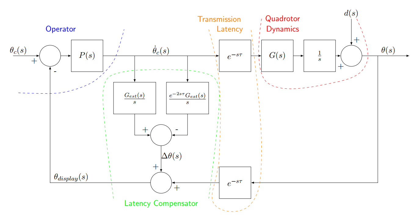
The block diagram shows an operator who decides an angular position command, compares this with the angular position displayed to them and determines an angular rate command as a response. The angular rate command is sent to the vehicle whose dynamics are applied along with disturbances to find the vehicles true angular rate. The vehicles angular rate is integrated to give the true vehicle angular position, which is sent back towards the operator. A transmission delay is applied and then the augmenter modifies the received vehicle angular position to figure out what to display to the operator.

The closed loop command and disturbance responses can be found from the block diagram.

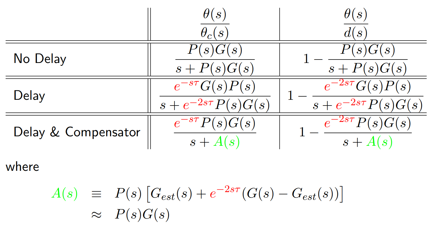
Starting with the no delay case, this is the classic complementary sensitivity function, with the 1 on the denominator replaced by s due to the integrator in the vehicle dynamics (which has not been included in G(s)). The disturbance response is the sensitivity function (written slightly differently for comparison later, with the unity disturbance response attenuated by a command response) with the same change in denominator for the same reason.

Moving on to the case with a delay (but without a compensator) the numerator is multiplied by the one-way latency. This is intuitively explained as the operator’s commands always taking some time to reach the vehicle. The delay in the numerator is annoying, but it only shifts the response in time, it doesn’t change what the response is. The delay in the denominator is much more nasty. This delay arises from the operator being unable to see the effect of their commands for the past 2τ time. Adding the delayed term to a term without any delay makes the response nonlinear and overall a headache. Similar arguments can be made for the disturbance response denominator. The disturbance response numerator is multiplied by a round trip delay term as the fact that there is a disturbance must be transmitted back to the operator, who then forms a response which is transmitted back to the vehicle.

Now we discuss the effect of the latency compensator. The latency compensator has no effect on the numerators, but the term in the denominator with a delay becomes A(s). A(s) contains the delay that was experienced previously, but it now multiplies (G(s) – G_est(s)). If the model of the system dynamics G_est(s) is sufficiently close to the true dynamics G(s), then A(s) will approximate P(s)G(s), and the denominator of the compensated system will approximate the denominator of the system without delay.

I obtained an accurate model using the MATLAB tfest function, which creates a linear model of a system from recorded inputs and outputs. I did this on the roll pitch and yaw axes of a rate mode quadrotor. System identification is not the focus of this article, but steps were taken to ensure that the model was accurate at a wide range of frequencies, and that overfitting did not occur. A number of flight logs were obtained and a model was fitted from all but one excluded log which was used for verification. This process of exclusion for verification was repeated for each log. The excluded log was also used for simulating the compensator (see below) to ensure a fair test. For implementation a model was fitted to all of the recorded logs.

An accurate model of the vehicle’s dynamics is needed, in reality the model will not be perfect. An important result that I found as part of my thesis was that the error in the displayed vehicle position does not grow with time and that any large momentary error will only persist for a duration of 2τ. I also simulated the compensator on logged flight data, with results consistent with the error not growing with flight time. The simulation also showed that the error in the predicted vehicle attitude was centred around zero and for a 1000ms latency had a standard deviation of about 1 degree, plenty accurate for a human pilot.

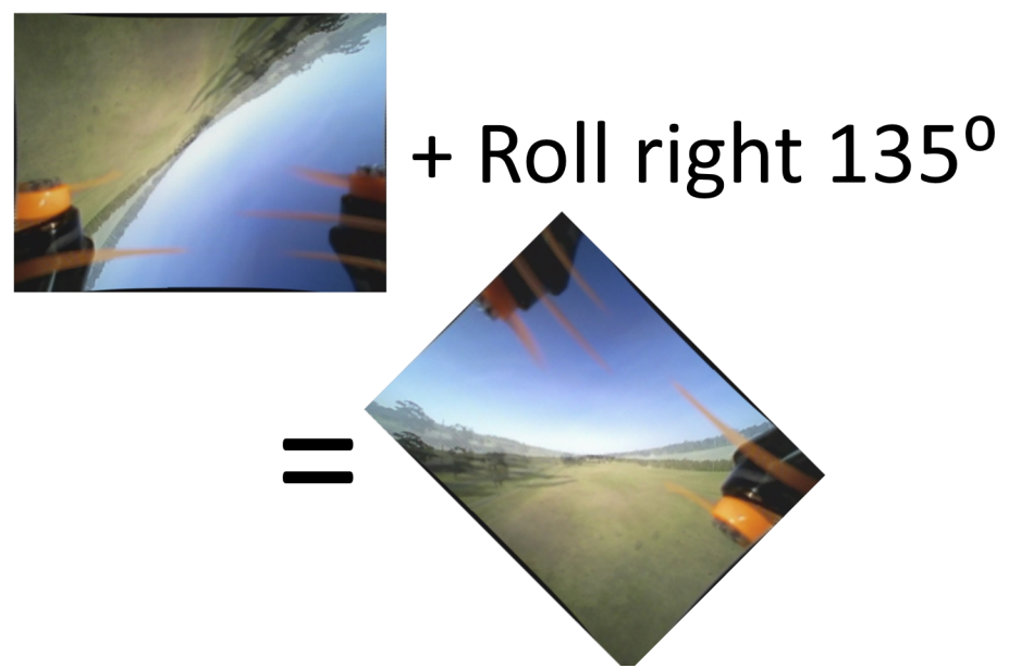
The feedback that I am choosing to augment is a video feed from a fixed camera onboard the vehicle. When the vehicle rotates, so does the camera and so does the view that the camera records. The pixels within the camera view can be mapped to light being received from a particular direction at the camera, and the camera’s rotation changes this mapping. The simplest implementation is to first calibrate the camera (remove lens distortion) and then rotate about its centre for the roll axis and translate (an approximation) it horizontally and vertically for the yaw and pitch axes. The following image shows a basic example of the compensator predicting that the vehicle will roll by 135 degrees over the delay time. This roll angle acts to rotate the video feed that is being received so that the pilot can see the vehicle’s attitude when their current command will arrive.

Implementation

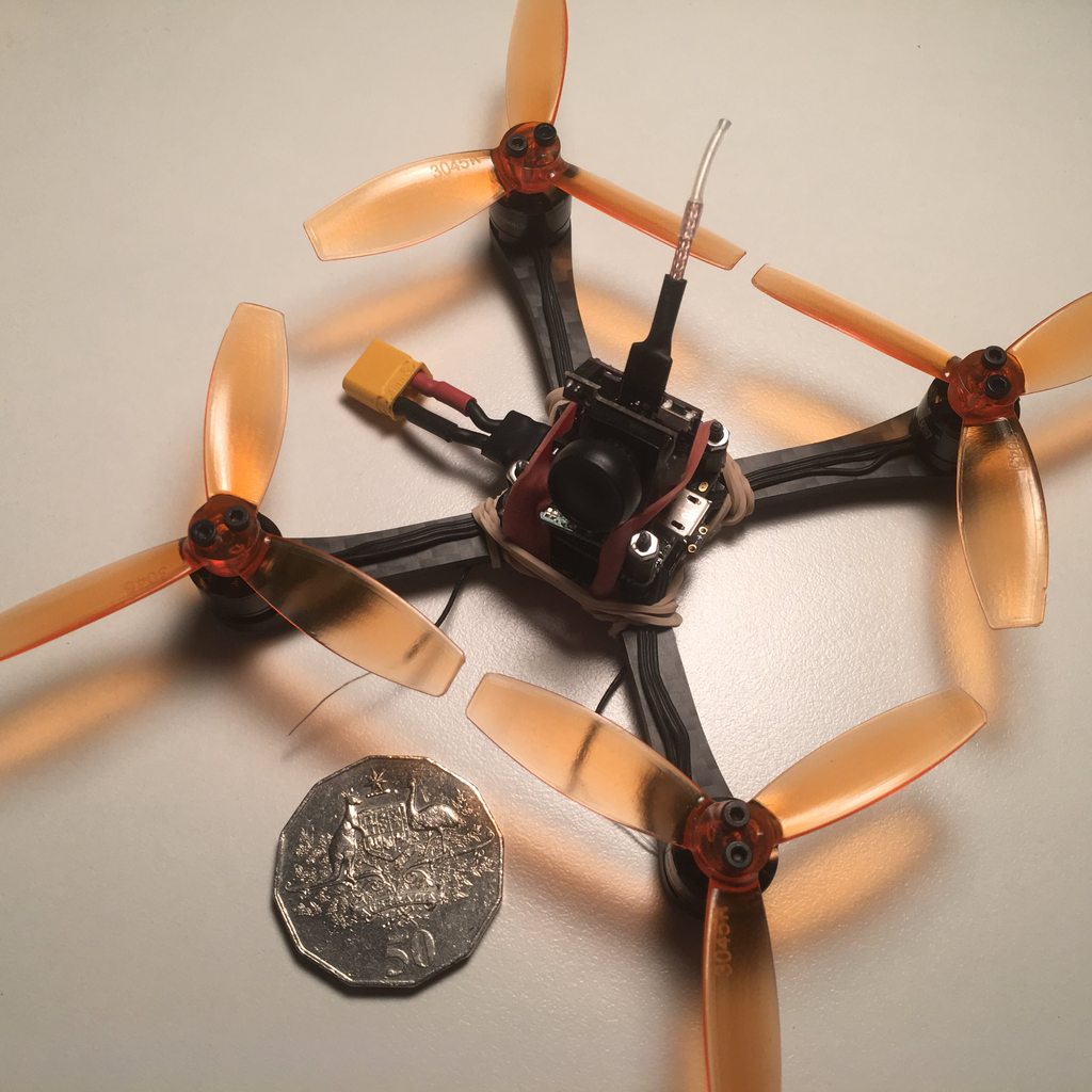
I chose to implement for a micro quadrotor flown in rate mode. Rate mode is the most primitive flight mode available on quadrotor platforms (unless you count the qwopcopter!) and does not self level, so without the operator’s influence the vehicle will rapidly destabilise and crash. Rate mode is also one of the most difficult to fly modes, with most operators unable to maintain control when flying for their first time (even the cheap plastic stuff you get from the bargain bin usually flies in a stabilised mode). The advantage of rate mode is that it permits the largest set of possible manoeuvres. Here is an image of the kind of micro quadrotor I am discussing, with an Australian 50 cent piece for scale (~32mm diameter, one of the largest coins in circulation).

With the vehicle sorted, the next step was to implement the latency compensator in real time. In my mind this consists of four main tasks; I/O of commands and feedback, real time system modelling, finding the vehicle state change and image warping. The first step is to select an environment. The Node.js environment is an event driven asynchronous javascript environment designed for scaleable I/O in server applications and real-time interactive internet applications. The Node.js backend is in C/C++ which permits calling C libraries from within Node.js (most conveniently through pre-written packages obtained using the Node Package Manager (NPM)). While my implementation works only locally, the Node.js environment is meant for internet applications, so adding functionality to transmit between two computers running Node.js environments should be straightforward.

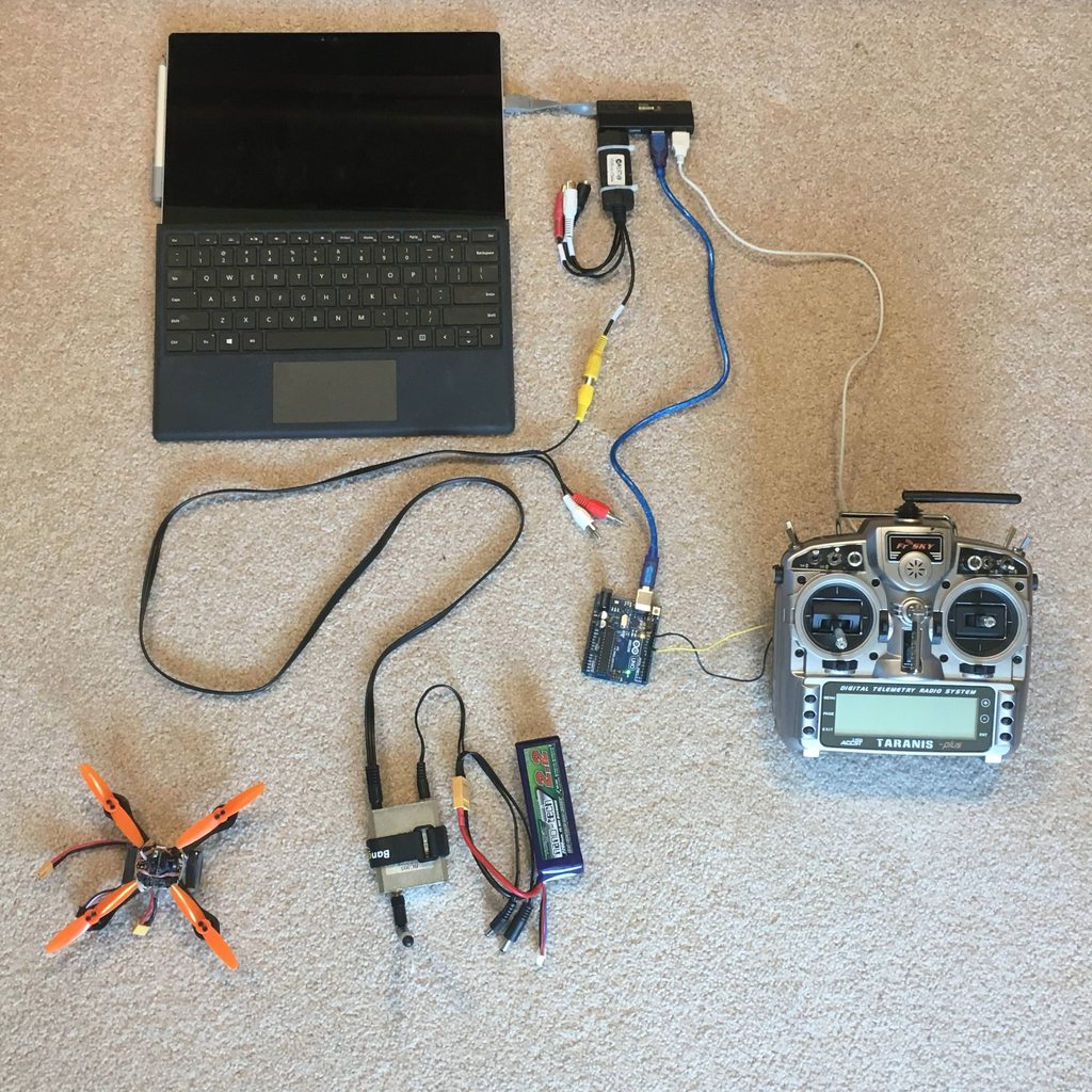
The I/O of commands and feedback needed to allow the real time model to read commands as they were given, as well as permit adding a delay before transmission. I used my FrSky Taranis X9D running a recent version of OpenTx to control the quadrotor. OpenTx broadcasts the first 8 channels as a usb joystick through a serial port in the back of the hardware, which is conveniently read by a Node.js package. A delay is applied to commands in the Node.js environment before they are sent back to the radio as a buddy box PPM signal (generated by an arduino) for broadcast to the vehicle. The video feedback is received over a typical 5.8GHz receiver as a composite video signal and is input to the computer via a USB digitiser, so that the video feed looks just like a webcom to the computer. Here is an image of all the hardware I used.

Running the model in real time presented a few challenges. The Node.js environment has a scheduler, which allows specifying a function to be called at regular intervals. This works great except that there is no guarantee that the interval you get will be the one you specify. Every now and then, your function which updates the vehicle state every 5ms will not be called for 50ms, as well as vary around the 5ms mark! A variable time step is needed, with a check to make sure that the time step is not so large as to make the model unstable. The continuous time state space model is converted to a discrete time state space model at each function call. With the vehicle’s angular rate the angular position is propagated using quaternions with a simple euler step process. Care must be taken to ensure that when the system model is queried that the state returned is current to the time of query or when the angular rate commands change.

The vehicle state change is calculated by storing the simulated vehicle states for a short time (in a circular queue for efficiency) and then comparing the vehicle state at the current time to the one at an earlier time. Because the vehicle state is only stored at discrete times, a linear interpolation is made between the closest two vehicle states stored at an earlier time and the state at the current time.

Image warping is performed using the OpenCVlibrary, a Node.js interface for which is available on NPM. This interface allows it to be called from JavaScript, but run in precompiled C (for speed). The most basic implementation has been used, with the picture displaced horizontally and vertically according to the vehicle attitude delta multiplied by the pixels per degree according to the resolution and field of view. Roll is achieved by rotating about the image centre (after translation for the yaw and pitch axes).

Results

As you may have seen at the start of this article, it works. The footage at the start of this article was the test pilot’s first attempt at flying with the compensator, so its success is consistent with the vehicle’s response matching the response with no latency (as suggested by the transfer functions). Flight testing was performed in three main modes, without latency, with latency and with latency and compensator.

When a latency was applied, even 500ms made the vehicle extremely difficult to fly, as seen in the flight below.

The motion seems reminiscent of pilot induced oscillation, though caused by a delay in seeing the response to pilot input.

Applying the compensator, the vehicle can be flown with up to a 1000ms latency, even permitting flips such as this one (shown in slow motion).

This slow motion flip is useful for understanding how it works and what is going on. The first 3 seconds show the operator commanding the flip. The picture rotates so that the operator can see the effect that their commands have. Some time later, the vehicle begins to actually perform the flip, and the camera’s view is rotated back the other way so that the horizon appears stationary. You may notice that the horizon dips substantially from level, which is due to the compensator only accounting for latency that I have introduced, and not for any latency in the various data interfaces. I have since measured this latency (by analysing the video recordings) and accounted for it, resolving this issue.